
Prepare Your Data For Analysis: Load Data With Spoon
Note: The instructions described here is learnt and utilized while working on the Clouds & Concerts project at University of Oslo in close collaboration with Xin Jian, Johannes Bjelland og Pål Roe Sundsøy under supervision by Arnt Maasø. The credit for methodology and SQL ninja tricks is therefore to be attributed to all members of the fantastic stream team. Inconveniences or mistakes are solely my own.
Technical set up
We chose to use Amazon as a solution for doing our data-analysis. Amazon Web Services provides both virtual computers, databases and storage in the cloud. All services are scalable so data loading and manipulation computer can be put dormant when idle, and the database can be scaled up when doing complex and data-intensive operations.
DSV files – choosing delimiter
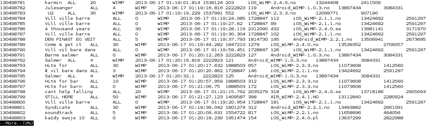
When moving large database files between two different servers in different organisations the standard way of exchanging data is through flat text files. The flat text files may have a structure e.g. XML or JSON, but in n the case of working with relational databases where all entries, or rows, have the same number of attributes, or columns, DSV is a convenient format. DSV is the abbreviation for delimiter separated values, and is a format where each attribute and each entry are separated with an assigned delimiter token. The most frequent delimiters are comma between attributes and newline between entries. This format is known as CSV.
When choosing delimiters, it is important to find a character that is not found in the data values. We chose to use tab as delimiter. To save space and transfer cost the files should be zipped (NB: the .zip-container supports only upto 4GB. If you have any larger files, use .gzip or .tar.gz).
Data delivery S3 bucket
Amazon’s Simple Storage Service (S3) is an easy way to retrieve data, either by using a client or using the web-interface accessible through the AWS console. All kinds of files may be uploaded to S3 including zipped or tar.gz-ed files. Files can easily be uploaded and downloaded to and from S3 by those who have access, and the web-uploader supports large files. You don’t have to define predefined storage space either since this is allocated on the fly.
Using Pentaho Spoon for loading
The software company Pentaho provides good tools for working with data-analysis, and part of their suite is the ETL-tool (Edit, transform, load) Spoon. This also comes in a community edition which can be downloaded from their homepage. The tool is built on Java so it can be run on different platforms. Once installed, use the terminal to navigate into the ‘data-integration’ folder, then set execution rights and run ‘spoon.sh’. This should open the spoon ETL-tool.
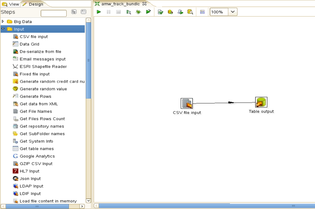
In Penthao you can make a transformation for each table you need to transfer, alternatively you can join more transformations together in jobs. To do a basic transfer of data from CSV, or other delimited files, to a database server you will need to use two modules: CSV file input and table output.
Set up a super-easy transformation to load csv to table
In the Pentaho, the convenient module CSV file input can be used for reading data from delimited files. 1: Use the file finder to select the file, set the delimiter and enclosure (e.g. if the strings are prepended and appended by quote marks). If you have a file dump where the header row is present, tick of this option. 2: The CSV file input module can try and determine the format of the various tables based on the data in the files. Use the ‘Get Fields’ option, and select a good sample size to determine the format.
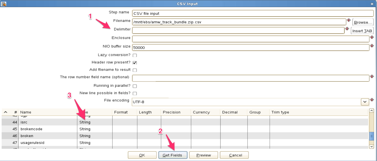
Loading tip: represent values as strings.
If you have a file with a high risk of data errors, for example a file where the columns overflow, I usually set the fields to text, using the functionality where I can define variable data-type (3), and make sure the length is large enough to encompass the data. This enables us to do the changes, and alterations of data format on the database server once the data is loaded. Most data can be represented in a string. Both “12354”, “182,54” and “01/08/1986 00:00:00,000000” can be represented as a string, but the first example can also be an integer, the second a real or float, and the third a timestamp. We can parse the data when we have them loaded into our SQL-database. You can adjust the type in the CSV file input module.
Use Table Output to write read rows to SQL-server
The other Pentaho module needed for this basic transformation is the Table output. Once Pentaho is configured with valid database configuration, this module can access the database directly so you can select to which table to write the data. First drag a line between the CSV Input module to to the Table Output to get the data connection. Then select output database/target schema and target table . If you have setup the table structure through a DDL (The Data Definition Language – The structure of the tables) you can map the fields from the CSV file input. In the database field tab you first select ‘Get fields’ to get the fields found or created in the CSV input module. Then select either ‘Enter field mapping’ if you have the full DDL loaded on the database or ‘SQL’ to create the DDL followed by ‘Enter field mapping’ (see tip below). Once the table is connected and the fields from the input data is connected to the fields of the database you are ready to run the transformation. Return to the workbench and press the play symbol on the top of the transformation tab.
Table loading tip: Let Pentaho deal with DDL
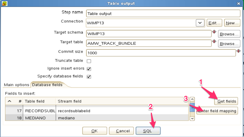
Once you have defined a connection by making a line between the CSV file input and the Table output, you can load the fields as they are stored in the flat CSV file using the ‘Get fields’ button (1). If you already have a defined table definition you can go straight to the mapping (3), but if you don’t have a DDL or you want the database table structure to follow the field definition you declared in the CSV file input you can use the SQL button (2) to get Pentaho to create the DDL and execute this on the database. To be able to do this you first have to create a table for the ‘target table’ field to be filled out. The trick is to know that you only have to fill in one variable when you create the target table e.g. execute the command “CREATE TABLE ALMOST_EMPTY_TABLE (ID_COLUMN INTEGER)” on the database, and let Pentaho deal with creating the rest. After running the SQL, you can map the fields (3) and then run then transformation.
Validate that the data is loaded into the database.
Check the number of loaded rows
In Pentaho Spoon, the transformation will have a step matrix when running where you can monitor the progress. During the load and upon completion the total number of rows will show here. To be sure that all data is loaded, or to get a number of how many rows that was dropped you can read this from the step matrix, but also by double checking the number of lines in the CSV file and the number of rows in the database table. The number of lines in the CSV file can be found by using the command “wc -l filename.csv” in the folder where the CSV files are stored (if the file have a header subtract the result by one), and compare this to the number of rows in the loaded table using “SELECT count(*) FROM tablename”.
Your data is now loaded into the database.